Excel - Compare two tables using COUNTIF

Do you have two tables (lists) in Excel, perhaps one is newer or you suspect it is different? You'd like to compare the two tables and see the differences easily? There are a few ways to do this, here I'm going to show how the COUNTIF function can be used, I've found it to be quick and easy to use.

Example
The following is an example where I have two tables in one Excel worksheet. You could have these tables in different worksheets of course. You also don't need to use Tables, this example would also work with ranges. It's just an example, I hope it is helpful to you:

The tables are named Table1 and Table2.

 

Table2 has less rows, only 1714 compared to 1718 in Table1. The question is, which rows are missing?

Enter a title to create a new column (above), a new table column will be created (below).

In the first cell in the new column you can enter the COUNTIF() function.

Enter:

=COUNTIF(Table2[Town], A3)

This means that we want look in the Town column of Table2 for whatever is in A3 (Table1). For example, it will look to see whether "Ampthill" is present in Table2 or not.

Because you entered the function into a column in a table, it'll replicate the formula all the way down. As you can see in the above example there is a result in each row of the column 'In Table2?'. COUNTIF() returns the number of times it found what it was looking for. Therefore you can see that on row 20 there's a zero, this means that "Ascot" could not be found in Table2.

Filter

Filters are automatically available for Tables, this makes it easy to see those results that are zero:

Filter the 'In Table2' column for all the zeros (where it did not find anything in Table2).

Enhance the look

For something quick the 0 or 1 is fine. If you want to share this with a others then you could tidy it up. Here's one way to do this:

Change the formula, add the surrounding IF() statement to set a Yes or No result. 

=IF(COUNTIF(Table2[Town], A3),"Yes", "NO!!!")

Having "NO!!!" makes it easier to spot where Table2 is missing this item.

Conclusion
This is just one way to compare data in two tables in Excel. It's nice and quick, I'm sure it can help anyone who just needs to quickly understand which rows are missing from a data set. 

I used the Excel 365 version as of August 2020 for this article. As the COUNTIF function is not new, I am sure this solution will work in older version of Excel too. That's another reasons it's a good choice.

PowerPoint - Turn off Design Ideas

Every time I paste a screen shot or anything into PowerPoint (the 365 version, June 2020) a pane appears to the right titled Design Ideas.

PowerPoint Design Ideas pane

This Design Ideas pane might be of some use but so far it has just been very annoying. It takes up space on the screen, especially when I'm working on a laptop. I don't need this distraction. 

Turn off Design Ideas

The following explains how to switch it off for good:

Click File | Options | General 

Click to disable Automatically show me design ideas

Click OK

If by any chance you do want an design idea from PowerPoint, you can click Design | Design Ideas (right most button on the Design menu).

How to use a Data API with Excel

A Data API is a way of easily accessing data. The Data API comes in the form of a URL web link. Software applications can use that link to download data. In this article we'll use Excel to download some data using a free Data API. 

Example scenario

I would like a list of all the countries in the world and their 3-digit ISO codes. I might want to use this information to combine with my own data for analysis. I could of course go to Wikipedia and download the list but that would be a static list. What if any of the data is updated in the future? It would be great if I could click Refresh and get the latest information. This Data API will allow me to do that.

The following website provides a free Data API for country information:

https://restcountries.eu/

We'll use this Data API for our example here but there are many different Data APIs available. 

Instructions

In Excel click Data (menu tab)

Click From Web (or click Get Data | From Web)

Enter the Data API URL. In our example we'll retrieve only two fields of data; the country name ("name") and 3-digit ISO code ("alpha3Code"): 

https://restcountries.eu/rest/v2/all?fields=name;alpha3Code

NOTE: More data fields can be retrieved, just add a semi-colon and the field name. We will explore this more, later in this article.

Click OK and Power Query opens...

On the Transform tab click To Table

Click OK

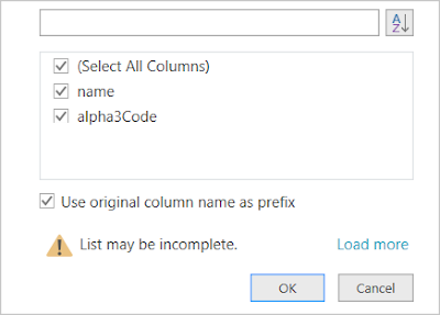
In the Column click the <-> icon (as shown above)

Click OK

Now you'll see the data in Power Query Editor:

Click Close & Load

A table will appear in your workbook:

The table is like any other Excel table. Use the data whichever way you like. 

Click Refresh to update/fetch the data from the Data API. 

More fields

The Data API URL from restcountries.eu can be modified to give more data. In principle this is how other Data APIs work too. Near the end of the URL it says fields=. The field names are listed with semi-colons to separate them. 

To fetch the country name and ISO code:

https://restcountries.eu/rest/v2/all?fields=name;alpha3Code

To fetch the country name, ISO code and capital city:

https://restcountries.eu/rest/v2/all?fields=name;alpha3Code;capital

To fetch everything in this data set:

https://restcountries.eu/rest/v2/all

Remember that the more data you retrieve, the slower it will be. Always try to restrict your request to the data you need.

TIP: If you want to test a Data API, paste the URL into your browser. If it's working you'll see all the data displayed (although difficult to read!). 

Excel version

I used Excel 365 (May 2020) in this example. However, it is likely older versions of Excel will work the same way or similar. Feel free to write comments below to help others.

Conclusion

Like many things this is easy once you know how. There are many public data sources available, just do a search and and you'll find many, sometimes free like the one here, others free but you must register (you need an ID to access the Data API) and others where you must pay (subscribe to a service). Of course you might also use this to easily access your own corporate data - ask your IT department! 

The best thing about Data APIs is that they can be updated easily and they are pretty easy to set up. I hope this article has been helpful, at least to get you started. 

If you want to learn more about APIs, have a look at this video, it's pretty good for beginners:

https://youtu.be/OVvTv9Hy91Q

Disclaimer

The Data API I used here as an example, it is just that, an example. I have no affiliation with that Data API site. I just used it because it was free to the public and had data that was good for this demonstration. If you find errors in the data please address any issue to that website and not to me. Everything I have written here is without guarantee, I'm just trying to help with this article :-)

Excel - Abbreviate huge numbers

Are you often working with very large numbers, possibly hundreds of thousands or even millions? Those numbers can become very long and difficult to read. There's an easy way to format them in Excel so they appear abbreviated. For example, 100,000 would appear as 100K. Here's what to do:

In the above example we have a couple of huge numbers. Select both cells, right click and click Format Cells.

Click Custom

Enter:
[>999999]#,,"M";#,"K"

Click OK

Now the numbers will appear abbreviated:

If you use pivot tables, this is invaluable. You can format the measures (Values) to be abbreviated just as above. Click the down arrow on the measure in the Values box, click Value Field Settings, click Number. This brings up the Format Cells window. Add the Custom template as explained above. Whenever you use that particular measure all the numbers will be formatted with this abbreviated format.

Excel - There are too many records to complete this operation

In Excel I was working with a pivot table. The following message popped up:
"There are too many records to complete this operation."

Solution
Click Analyze (or Options in Excel 2010)
Click Fields, Items & Sets
Click Solve Order

If you have something listed, it is probably causing the problem. Delete it, then try working with your pivot table again, all should be well.



NOTE: I've tested this with Excel 2013 but it should work the same way with other versions.

Excel - date and time stamp keyboard shortcuts

There are many situations where it makes sense to enter a time stamp or today's date into your worksheet. Of course there are functions such as TODAY() and NOW() but these will recalculate automatically. If you want just to input a date or time, there's a couple of handy keyboard shortcuts you can use:

Press Ctrl-: (control and colon) to insert today's date.
Press Ctrl-; (control and semi-colon) to insert the current time.




NOTE: I've tested the above with Excel 2013 but it should work with other versions too.

Excel - split e-mail addresses in one cell to separate rows

In Outlook if you copy e-mail addresses from the To or CC lines you end up with something like this:

email01@address.com;email02@address.com;email03@address.com;

Paste the above into Excel and it's the same, all the addresses are in one line and in one cell. What if you'd prefer them in a vertical list like this:

email01@address.com

email02@address.com

email03@address.com

In this article we'll go step-by-step through the process of splitting the addresses from one cell into many rows. 

Instructions

Select the cell containing the e-mail addresses

Click Data | Text to Columns

Click Delimited

Click Next

Click Semicolon

Click Next

Each e-mail address will now appear in separate columns...

Select all the column cells of all the e-mail addresses (as shown above)

Press Ctrl-C to copy them

Click in a cell below (A6 in our example above)

Right click...

Click the Paste Transpose button (as shown above)

The addresses will now be listed on separate rows:

That's it!


Tidy Up
However, there's a space before some of them, if you want to tidy that up, use the Replace option as follows:

Click Home | Find & Select | Replace

In the 'Find what' box put a space, do not enter anything in the 'Replace with' box

Click Replace All

The following is the result:

Conclusion
I hope that was helpful. The above works fine in Excel 2013 but it's very likely to work in Excel 2010 and other versions too.

Add a custom colour to your default colour palette in Word and other Office applications

I'm currently using Office 2013 and there's a colour I use often in my documents, it isn't the usual blue, it is different from any of the blues provided with the Office applications. To get this special blue I have to add it as a custom colour using the colour code RGB 0, 144, 188. But I have to do this every time I open Word, for example.

After entering my custom colour it is shown at the bottom of the window in the Recent Colors, so I can quickly select it. However, when I close and reopen Word, my custom colour has gone. I have to enter the custom colour every time I start Word. It's the same story for the other Office applications.

I would like to have my custom colour available for all new documents I create. This can be very important, imagine your company has it's own corporate colours, shouldn't they be available to everyone as part of the standard colour palette? It's a bit much to expect user to enter custom colours using RGB codes for every document. Having the colours available easily will make the adoption of the correct colours much easier.


NOTE: I'm using Office 2013 / Word 2013 in my example here, in other versions you may find some differences but I hope at least this will help you find your way.


Solution for Word 2013
In Word, click File, New and Blank Page (or the template you would like to add your custom colour to)

Click Design

Hover the pointer over Colors to see which theme you are currently using - as in the example below:

In the above example I am currently using the Office theme.

Click Colors

Click Customize Colors (at the bottom of the drop-down list)

On the ‘Create New Theme Colors’ window, select one of the preset colours, in my example I will change Accent 5 because it is already close to the custom colour I want to add.

Click More Colors

Click the Custom tab

Enter the colour you would like, in my example RGB 0, 114, 188

Click OK

In the Name box change Custom 1 to the theme name that you’d like, in my example “Corporate Colours” and click Save.

Now your new colour is accessible for the current document (you can see it at the top of the menu - above). However, if you’d like it to be available for all new documents using this template, on the Design tab...

...and click Set as Default.

Here's what it looks like to actually use it:

Outlook 2013
Once you've created a new Colour Theme in one Office application, it'll show up in other applications. For example, when I am composing an e-mail the same colours will be available. In the screen shot below you can see the Options menu where the Colors menu is located.

Excel 2013
As with Outlook, the same is true but look on the Page Layout tab for the Colors option.


Powerpoint 2013
It is a little different here, go to the Design tab. Click the expand button on the 'Variants' box:

There is the usual Colors option to select from.

Deploy to other computers
I am sorry but I have not done this myself so I cannot provide a full explanation here. However, I did discover that the new Colour Theme I created and named "Corporate Colours" in Word, was stored as an XML file like this:

C:\Users\<username>\AppData\Roaming\Microsoft\Templates\Document Themes\Theme Colors\Corporate Colours.xml

I copied the Corporate Colours.xml file to the same folder on another computer with Office 2013. I opened Word, clicked Design, looked on the Colors button and yes, my Corporate Colours option was there at the top of the list. This means you could distribute this file to all workstations on your network to provide the corporate colours to everyone.

I also found the following page on the subject, using Group Policies:
https://technet.microsoft.com/en-us/library/cc178992(v=office.15).aspx

I hope that helps!


Conclusion
If you are using a particular colour often, this really is a great little time saver. If you are using a whole palette of colours, perhaps a corporate colour scheme - this is essential. I say essential because expecting users to enter RGB numbers is a lot to ask them. They will make mistakes or forget. Customising the colours available in Office applications is best and as you can see here, it is not difficult.


Reference
Microsoft Office Change a Theme
https://support.office.com/en-us/article/Change-a-theme-and-make-it-the-default-in-Word-or-Excel-c846f997-968e-4daa-b2d4-42bd2afef904

Deployment
https://technet.microsoft.com/en-us/library/cc178992(v=office.15).aspx

Deploy templates
http://www.thewindowsclub.com/custom-templates-installation-location-office

Excel 2013 - Compare two spreadsheets

A few years ago I wrote an article explaining how to use a third-party tool to compare worksheets in Excel 2010, click here to read it. Recently I wanted to do the same but using Excel 2013 and I was pleasantly surprised to find there is a special tool included with Office 2013 that can do this job. The tool is called Spreadsheet Compare, the chances are that if you are an Excel 2013 user, you already have this tool on your computer.

Using the Windows search (press Win-S or click Start and type in the search box) do a search for "spreadsheet compare", it'll come up, run it and you'll see it's a nice straightforward little program. Just click the Compare Files button and enter the Excel worksheets you'd like to compare.

In my example above I compared two files and you can see in the lower middle window three changes are listed. One is a spelling correction of Woburn and I've clicked on it - then in the two windows above showing the original worksheets, it moves to that position to show the difference.

Also, Spreadsheet Compare can be started from the INQUIRE tab from within Excel 2013. Just make sure you have the worksheets you want to compare open before running it from there.

For more details including a step-by-step explanation please see the Microsoft page, they've done a good job already so there wasn't a need for me to redo it here. Click the following link (last accessed 17/01/2017):
https://support.office.com/en-us/article/Basic-tasks-in-Spreadsheet-Compare-f2b20af8-a6d3-4780-8011-f15b3229f5d8

Excel - Calculate week days from dates

Often in Excel dates are used. In this article we'll see how we can list the corresponding day of the week using a formula. We'll use the CHOOSE() and WEEKDAY() functions, here's how:

=CHOOSE(WEEKDAY(A2),"Sunday","Monday","Tuesday","Wednesday","Thursday","Friday","Saturday")

Using the above formula you'd need to have a date in cell A2, the WEEKDAY() function will pass the number of the day of the week to the CHOOSE() function and it displays the corresponding text (in numerical order). The following screen shot shows the formula in action.

This was tested in Excel 2013 but it is likely to work in any version of Excel.



Update 9th May 2016
If the date is missing it'll be zero, the result of the above function in column B will be "Saturday" - which makes no sense. To improve the above formula so if there are any missing dates the Day column shows nothing, use the following:

=IF(A2="","",CHOOSE(WEEKDAY(A2),"Sunday","Monday","Tuesday","Wednesday","Thursday","Friday","Saturday"))

The above, in English words means, if the A2 cell is empty do make the cell (Day cell) empty. But if there's something in A2, calculate the day and display it (in the Day cell).

Excel - Repeat All Item Labels in a pivot table

Introduction
When working with pivot tables, especially OLAP pivot tables, it's often the case that I have needed to flatten the pivot and copy the data to a new sheet to create a new table (a 'flat file'). One important part of this is to fill in the data labels of the rows.

On the Design tab, click Show Report in Tabular Form
Previously to fill in all the labels, on each column I was right clicking, Field Settings | Layout & Print | Repeat Item Labels:

However, this only works for one column at a time.

Repeat All Item Labels
The following is a better way of doing it, below we repeat all the item labels for the whole pivot table in one go with just a couple of clicks:

Click on the pivot table
Click Design
Click Report Layout | Repeat 


Conclusion
It is strange that Microsoft put the two variations of this function in different places. However, it was my mistake not to notice this earlier. Maybe you didn't notice it either? If so I hope this article has helped you.


Excel Version?
Excel 2013 and 2010.

Excel - A PivotTable report cannot overlap another PivotTable report

In Excel 2013 click on an existing pivot table and click Refresh to refresh the data in the pivot table. The following error message may appear:
A PivotTable report cannot overlap another PivotTable report.

Reason
Somewhere in your workbook there are two pivot tables on one sheet that are close together. When you refresh one of those pivot tables 'grows' in size (because of a change in data perhaps).


Solution
The pivot table you clicked refresh on may not be the one that's causing the trouble. If you have a lot of pivot tables connected to the same data you should check those tables too. Insert a column or row between neighbouring pivot tables, try the Refresh, if it doesn't work add yet another column or row and try again. You will find a neighbouring pivot table that was causing the trouble.

For me, I found that I had a Grand Total column off on a pivot table but when I refreshed it turned on, causing it to bump up against another pivot table.

To avoid this issue altogether make sure there is at least a couple of columns/rows between pivot tables or place them on separate sheets if you can.

IMPORTANT: If you click Refresh on a pivot table that is on its own on one sheet and it gives the above error it is because clicking the Refresh button tries to update all pivot tables connected to that one data source. Therefore somewhere else, on another sheet perhaps, you must have two pivot tables side by side and one is growing in size with the refresh and 'hitting' the other one. Therefore if you get this error, look through all your sheets, not just the one you are working with.


Excel Version?
I experienced this issue with Excel 2013 but I presume it will be the same with Excel 2010 and maybe even earlier versions. If anyone has additional information please feel free to add your comments below.